Quantum Mechanics Introduction

— 1. Motivation —

Unlike we did so far in the previous posts first we'll begin to study Quantum Mechanics by mentioning some of the experiments that motivated the reformulation of Classical Physics into the body of knowledge that is Quantum Mechanics. Also we'll spend more time explaining our initial formulations.

— 1.1. New results, new conceptions —

Anyone that has ever realized an experiment before knows that if one wants to know anything about a system that is being studied one needs to interact with it. In a more formal language one should say: "The act of measuring a system introduces a disturbance in the system". Thus far we've used the concept of mechanical state on our analysis of physical systems. A more critical eye to the concept of reveals the following:

1. In principle the disturbance can, in some cases, be made as small as one wants. The fact that exists a limit in our measuring apparatus lies in the nature of the apparatus and not in the nature of the theory being used.
2. There exists some disturbances whose effect can't be neglected. Nevertheless one can always calculate exactly the value of the effect of the disturbance and compensate it in the value of the quantity that is being measured afterwards.

Thus one can say that our very successful Classical Theory of Physics is casual and deterministic. Despite its many successes our Classical Theory of Physics had a few dark clouds hovering over it:

• Black body radiation.
• Photoelectric effect.
• Rydberg–Ritz combination principle.
• The existence and stability of atoms.
• Stern-Gerlach's experiment.
• Electron diffraction.
• ...

The persistence of these experimental results and the failure of accommodating them in the classical world view indicated that a revision of concepts was needed:

• Corpuscular entities were demonstrating wavelike behavior.
• Wave entities were demonstrating pointlike behavior.
• There exists a statistical nature in atomic and subatomic phenomena that seems to be an essential characteristic of Nature.
• Nature's atomic nature (no pun intended) implies that the process of measure has to be thought over: some disturbances can't be made arbitrarily small since there exists a natural limit to how small a disturbance can be made.

— 1.2. Double-slit experiment —

In order to make our previous discussion more concrete we'll look into a particular experiment that makes it clear how disparate are the two world views that we've been discussing.

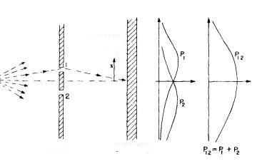
— 1.2.1. Double-slit and particles —

Suppose an experimental apparatus which consists of a wall with two opening and a second wall that will serve as target. A beam of particles is fired upon the first wall. Some of those particles will hit the wall and of some will pass through the slits and hit the second wall.

The particles that pass through slit $ {1}$ are responsible for the probability curve $ {P_1}$ while the particles that pass through slit $ {2}$ are responsible for the probability curve $ {P_2}$. The resulting probability curve, $ {P_{12}}$, results from the algebraic sum of the curves $ {P_1}$ and $ {P_2}$.

— 1.2.2. Double-slit and waves —

Now if we direct a beam of waves on the same experimental apparatus the pattern one observes in the second wall is:

 

Now what we'll study is the intensity curve. The intensity curve $ {I_1}$ is the result one would observe if only slit $ {1}$ was open, while the intensity curve $ {I_2}$ is what one would observe if only slit $ {2}$ was open. The resulting intensity is given by the mathematical expression $ {I_{12}=|h_1+h_2|^2= I_1+2I_1I_2 \cos \theta}$. The last term is responsible for the interaction between the waves that come from slit $ {1}$ with the waves that come from slit $ {2}$ which ultimately is what causes the interference pattern one observes in the second wall.

— 1.2.3. Double slit and electrons —

Now that we familiarized ourselves with the behavior of particles and waves under the double slit we'll study what one observes when we subject an electron beam through the same apparatus. Experimental results show conclusively that electrons are particles so we're expecting to see the same pattern that we saw for macroscopic particles. Nevertheless this is what Nature has for us!: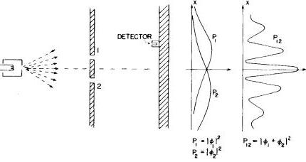

In the case of electrons Nature forces to think again in terms of curves related to wave phenomena. But unlike macroscopic wave phenomena this aren't curves of intensity but they are curves of probability. This introduces an apparent oxymoron since probability curves are a concept that is intrinsic to particles while an interference pattern is intrinsic to waves...

In order to explain what we're observing one has to assume that each probability curve $ {P_i}$ is associated to a probability amplitude $ {\phi_i}$. In order to calculate the probability one has to calculate the modulus squared of the probability amplitude, $ {P_i=\phi_i^2}$. Thus one has to first calculate the sum of probability amplitudes of an electron passing through slit $ {1}$ or passing through slit $ {2}$ and only then should we calculate the modulus squared of the probability amplitude of an electron passing through slit $ {1}$ or slit $ {2}$:

$ \displaystyle P_{12}=|\phi_1+\phi_2|^2$

— 2. Basic concepts and preliminary definitions —

After our initial discussion I suppose that you understand why physicists had the need to introduce a new paradigm that made sense of what's happening in the atomic and sub- atomic level. Now it's time to introduce our usual initial definitions.

Definition 1 An operator is a mathematical operations that carries a given function into another function.

As an example of an operator we have $ {\dfrac{d}{dx}}$ which a transforms a functions into its $ {x}$ derivative. As another example of an operator we have $ {2\times}$ that transforms a function into its double.

Definition 2 The linear momentum is represented by the operator $ \displaystyle p=\dfrac{\hbar}{i}\dfrac{d}{dx} \ \ \ \ \ (1)$

Definition 3 The energy of a particle is represented by the operator: $ \displaystyle E=i\hbar\dfrac{d}{dt} \ \ \ \ \ (2)$

Definition 4 For a free particle the following mathematical relationships are valid:$ {\begin{aligned} \label{eq:relacoesdebroglie} k &= \frac{\hbar}{p}\\ \omega &= \frac{E}{\hbar} \end{aligned}}$

— 3. Quantum Mechanics Axioms —

After this batch of initial definitions that allows us to know the entities that will take part in the construction of our quantum vision of the world it is time for us to define the rules that govern them

Axiom 1 The quantum state is defined by the specification of the relevant physical quantities and is represented by a complex function $ {\Psi(x,t)}$

Axiom 2 To every observable in Classical Physics ($ {A}$) there corresponds a linear, Hermitian operator ($ {\hat{A}}$) in quantum mechanics.

Axiom 3 Measurements made to an observable associated with the operator $ {\hat{A}}$ done on a quantum system specified by $ {\Psi(x,t)}$ will always return $ {a}$ where $ {a}$ is an eigenvalue of $ {a}$. $ \displaystyle \hat{A}\Psi(x,t)=a\Psi(x,t) \ \ \ \ \ (3)$

Axiom 4 The probability that a particle is in the volume element $ {dx}$ is denoted by$ {P(x)dx}$ and is calculated by $ \displaystyle P(x)dx=|\Psi(x,t)|^2dx \ \ \ \ \ (4)$

Axiom 5 The average value of a physical quantity $ {A}$, represented by $ {<A>}$, is $ \displaystyle <A> = \int \Psi^*\hat{A}\Psi \ \ \ \ \ (5)$

Where the integral is calculated in the relevant volume region.

Axiom 6 The state of a quantum system evolves according to the Schrodinger Equation. $ \displaystyle \hat{H}\Psi= i\hbar\frac{\partial \Psi}{\partial t} \ \ \ \ \ (6)$

Where$ {\hat{H}}$ is the hamiltonian operator and corresponds to the total energy of a quantum system.